Chapter 1 | Introduction
In this project we use raster and vector data on the form of cities to compare urban core morphologies across America. To do this, we aggregate street networks, building footprints, vegetation and population from a combination of open source resources. The result is a similarity score for cities, focusing on extracts of downtowns, allowing users to compare built environments across the country, along with twin cluster analyses to build categories of these environs. Motivating this analysis is the desire for a better way of comparing the focal areas in cities—the area where tourists visit, workers commute, and residents go out. If we are going to relate cities to each other, we want to look at the core—in several senses of the word. This is difficult to distill in a replicable, codable manner; we choose a method here but there are doubtless many others.
datasets
The bulk of these data come from osm via the osmnx interface. Building on past and recent work from Geoff Boeing, we determine if a city is flat or hilly, gridded or messy, dense or sparse, paved or planted, and how busy it gets at day and at night. Buildings, streets and their orientations are plotted below.
Measures of urban form
Oak Ridge National Laboratory provides information on daytime and nighttime population at a resolution of 100 meters, which we use to estimate how busy an area is, and whether or not people are concentrated on a few pixels or many. This also helps describe the character of an area: how many people are around changes your experience of it. Below we plot day-night variations for Manhattan according to this data.
Day-night variations
Finally, Google provides access to remote sensing data via its earth engine library. We use this interface to perform zonal statistics on satellite images in the cloud before exporting tabular data. This critically saves memory and allows us to perform computations across the country without committing rasters that size to working memory.
questions
The question we are trying to answer is how much variation is there across “Downtown America” and what patterns occur regardless of the state or region? Which cities are similar and which are different? In order to relate cities to each other, we create a similarity score for urban cores, associating each city with others by the character of its built environment. Further, clustering, including k-means and hierarchical, provides a way of checking the robustness of our similarity score: deviations in results between techniques signal less certainty in these relationships. We also build a tool for understanding—when twinned with mobility data—what kinds of downtowns are popular, which could be important as cities attempt to market themselves in the age of remote work, and a database that can be leveraged for future analysis.
methods
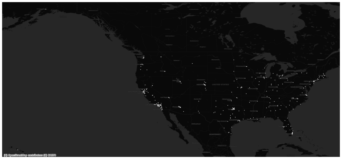
We scrape data on cities in the United States from wikipedia and estimate the downtown by geocoding for “City Hall” in each city name—so a query would be “City Hall, City of New York, New York, USA”. Most mapping and geocoding services fail with such vague language (MapBox and OpenStreetMap struggled in tests), so we use Google Maps. The sample is mapped below.
cities
With coordinates for each city hall, we use osmnx to select features within a given radius from them. With streets and buildings along with remote sensing data for each downtown (as I define it), we then perform a series of calculations to assess the form.
These include:
- Fractal dimension
- Network entropy
- Mean building size
- Street gradient
- Node density
- Mean edge length
- Daytime/Nighttime population
- Vegetation index
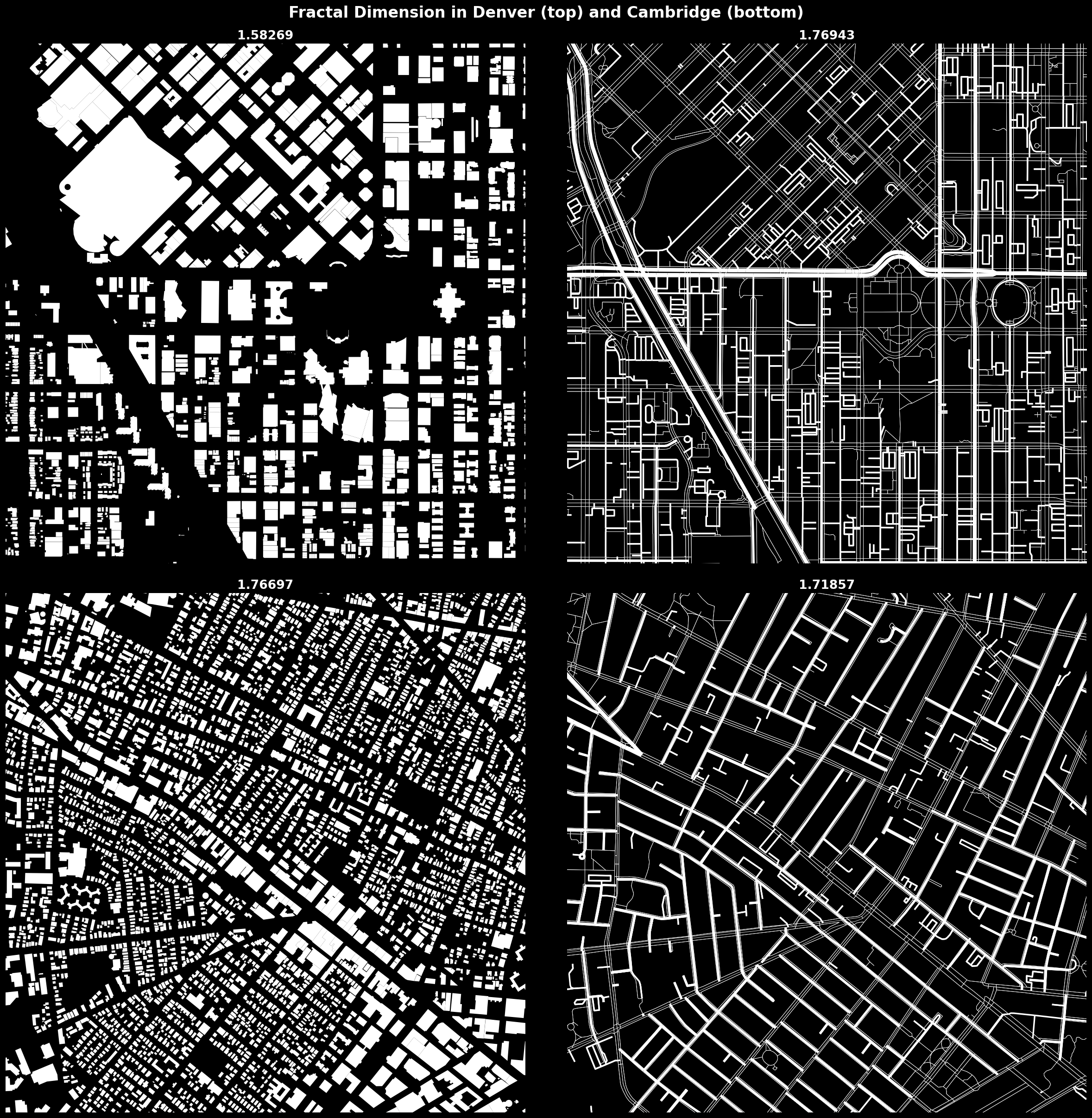
By way of example, we compute how repetitive a city is using a measure called fractal dimension, which roughly captures how much a city at a given scale is like itself at another scale: does a city look the same if you take bigger or smaller tiles of it? Fractal dimension is typically used in the study of urban growth, but here we are concerned with whether or not a city is assembled from a reproducible pattern or if each block. Because the form of a city is manifest in both its buildings and streets, we build a measure that includes the fractal dimension of both.
Fractal dimension by buildings and streets
In total, we gather 32 indicators of urban form, with minimum, maximum, and mean or median in several categories expanding the list from above. Not all are valuable in this analysis—and we attempt to reduce dimensionality in our data by aggregating variables—but they constitute a dataset that may be valuable for future studies.1
The last variable is grid index, which comes from a recent paper by Geoff Boeing; it combines the proportion of intersections that are four-way, the circuity of streets, and orientation entropy of streets—how much variation is there in a city’s bearings, between all streets on a single axis and no streets sharing an axis. We replicate his construction using the same measures and similar techniques from his paper, taking the geometric mean of these variables (after scaling) to produce a single index.
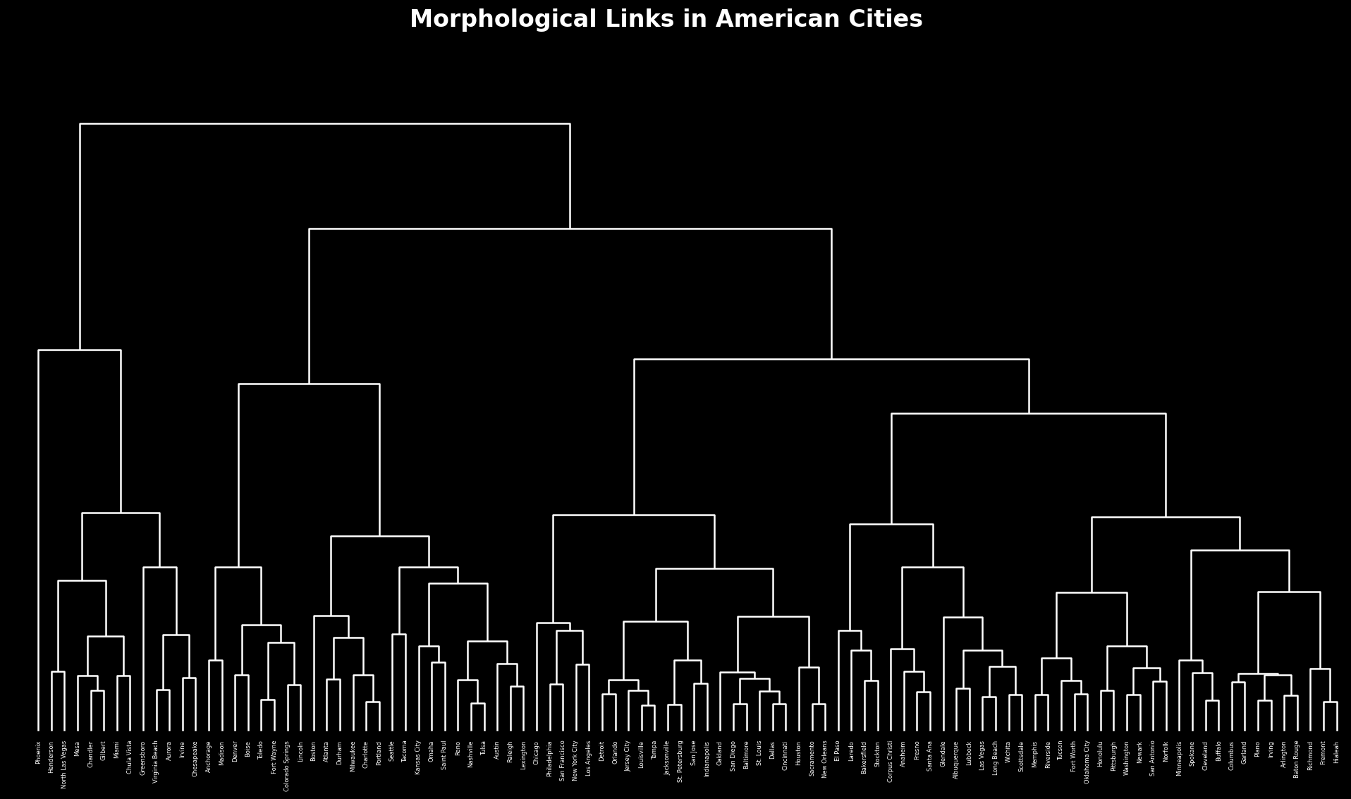
Finally, we use clustering analysis to make sense of the relationships between cities, with k-means to understand broad groups and hierarchical to understand narrow dyads or triads. The similarity score uses a k-nearest neighbors distance calculation, borrowing from sports analytics, allowing us to make tables of first, second, and third most similar cities for any given city. Cities that are closest together in a multidimensional space are more similar; cities farthest away are less similar.
results
The result is a series of insights into how similarity is distributed across the country and how similarity clusters among both class and location. We find that that many large cities in America like Philadelphia, Chicago and New York—cities on grids, with large commuter populations—are similar by these measures, and that cities like Denver and Boise are also related. The most dissimilar city in America, according to this similarity score and affirmed by hierarchical dendrogram, is Phoenix.
-
Note that because we are taking tiles of fixed area at each point, many of the above variables are already functionally scaled—the number of nodes and edges are also those number per 2000 * 2000 meter cell. ↩
Updated: